MATLAB Tutorial for Beginners
Tutorialspoint
Vectors
Full Matrix
Commonly Used Commands
clear
clc
close all
help
Vectors
Dot Products
Create random vectors $\mathbf{v}_1$ and $\mathbf{v}_2\in\mathbb{R}^n$.n = 1000000; v1 = rand(n,1); v2 = rand(n,1);Compute $\langle\mathbf{v}_1, \mathbf{v}_2\rangle$.
Method 1 Use the command
dot
a = dot(v1,v2);
Method 2 Compute the matrix product $\mathbf{v}_1^\top\mathbf{v}_2$.
b = v1.'*v2;
Question Which method is more efficient?
Matrix
Full Matrix
A small matrix \[ A=\begin{bmatrix} -2 & 1 & 0 & 0 & 0\\ 1 & -2 & 1 & 0 & 0\\ 0 & 1 & -2 & 1 & 0\\ 0 & 0 & 1 & -2 & 1\\ 0 & 0 & 0 & 1 & -2 \end{bmatrix}_{5\times 5} \] can be constructed by
A = [-2  1  0  0  0;
      1 -2  1  0  0;
      0  1 -2  1  0;
      0  0  1 -2  1;
      0  0  0  1 -2];
Sparse Matrix
A large matrix with lots of zero entries \[ A=\begin{bmatrix} -2 & 1 & 0 & \cdots & 0\\ 1 & -2 & 1 & \ddots & \vdots\\ 0 & 1 & -2 & \ddots & 0\\ \vdots & \ddots & \ddots & \ddots & 1\\ 0 & \cdots & 0 & 1 & -2 \end{bmatrix}_{10000\times 10000} \] can be constructed byn = 10000; A = sparse(1:n-1, 2:n, 1, n, n) + sparse(1:n, 1:n, -2, n, n) + sparse(2:n, 1:n-1, 1, n, n);or
n = 10000;
A = spdiags([ones(n,1) -2*ones(n,1), ones(n,1)], -1:1, n, n);
Question Which method is more efficient?
Linear System Solver
Create a matrix $A\in\mathbb{R}^{n\times n}$ and a vector $\mathbf{b}\in\mathbb{R}^n$.n = 100; A = rand(n,n); b = rand(n,1);
The linear system $A\mathbf{x} = \mathbf{b}$ can be solved by the backslash operator "
\".
x = A\b;
The accuracy of the linear system solver can be check via the maximal residual.
Residual = max(abs(A*x-b))
Application: Finite Difference Method for Numerical Differential Equations
A 1D boundary value problem of Poisson equation is given by \begin{equation}\tag{1}\label{Poisson} \begin{cases} \frac{\partial^2 u}{\partial x^2}(x) = f(x) ~\text{ on $[a,b]$},\\[0.1cm] u(a) = \alpha,\\[0.2cm] u(b) = \beta. \end{cases} \end{equation} In the following, we demonstrate a step-by-step implementation for solving the equation \eqref{Poisson} by using the central difference scheme \[ \frac{\partial^2 u}{\partial x^2}(x) \approx \frac{u(x+\delta x) - 2 u(x) + u(x-\delta x)}{(\delta x)^2}. \] First, we set up the domain $[a,b]$ and the array of grid points $\mathbf{x}=(x_1, x_2, \ldots, x_{n+1})^\top$, where $x_\ell = a + (\ell-1) \delta x$, for $\ell = 1, 2, \ldots, n+1$.a = 0; b = 5; n = 64; % number of intervals N = n+1; % number of points dx = (b-a)/n; x = (a:dx:b).';
Set up the right-hand-side function $f$ in \eqref{Poisson}, and the exact solution for comparison purpose.
u_exact = @(t) t.*cos(t);
f = @(t) -2.*sin(t) - t.*cos(t);
Set up the boundary conditions $\alpha$ and $\beta$ in \eqref{Poisson}.
alpha = u_exact(a);
beta = u_exact(b);
As a result, the equation \eqref{Poisson} is written into a system of equations \begin{equation}\tag{2}\label{LS} \frac{u(x_{\ell+1}) - 2 u(x_\ell) + u(x_{\ell-1})}{(\delta x)^2} = f(x_\ell), \end{equation} where $u(x_1)=\alpha$ and $u(x_{n+1})=\beta$ are given. The system \eqref{LS} is written as \[ L\mathbf{u} = \mathbf{f}. \]
L =   sparse(1:N-1, 2:N  ,  1, N, N)...
    + sparse(1:N  , 1:N  , -2, N, N)...
    + sparse(2:N  , 1:N-1,  1, N, N);
L = L/dx^2;
Define the index sets of interior points and the boundary points.
I = (2:N-1).';
B = [1; N];
Define the solution vector $\mathbf{u}$, and set up the boundary condition $\mathbf{u}_\mathtt{B}$. Then the equation \eqref{Poisson} is solved by the linear system \[ L_{\mathtt{I},\mathtt{I}} \mathbf{u}_{\mathtt{I}} = \mathbf{f}_{\mathtt{I}} - L_{\mathtt{I},\mathtt{B}} \mathbf{u}_{\mathtt{B}}. \]
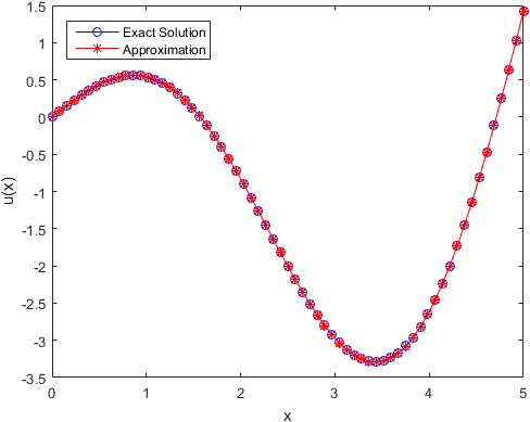
u = zeros(N,1);
u(B) = [alpha; beta];
rhs = f(x(I)) - L(I,B)*u(B);
u(I) = L(I,I) \ rhs;
Show the result.
figure
plot(x, u_exact(x), 'bo-', x, u, 'r*-');
xlim([a, b]);
xlabel('x');
ylabel('u(x)');
legend('Exact Solution','Approximation','location','northwest');
Check the maximal residual and the errors in $1$-norm, $2$-norm and $\max$-norm.
Residual  = max( abs(L(I,I)*u(I) - rhs) );
Error_1   = dx*sum( abs(u_exact(x)-u) );
Error_2   = sqrt( dx*sum( abs(u_exact(x)-u).^2 ) );
Error_max = max( abs(u_exact(x)-u) );

fprintf('Residual        = %e\n', Residual);
fprintf('Error in 1-norm = %e\n', Error_1);
fprintf('Error in 2-norm = %e\n', Error_2);
fprintf('Maximal error   = %e\n', Error_max);
Residual        = 1.998401e-13
Error in 1-norm = 5.151532e-03
Error in 2-norm = 2.621491e-03
Maximal error   = 1.956803e-03
Exercise 1 Try to increase the number
n, and see whether you could obtain a more accurate result.
Exercise 2 Try to change the exact solution
u_exact and the related right-hand-side function f, and see how the error varies.