Triangular Mesh
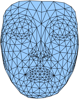
A triangular mesh $\mathcal{M}$ in $\mathbb{R}^3$ is composed of vertices \[ \mathcal{V}(\mathcal{M}) = \left\{{v}_k \equiv \left( {v}_k^1, {v}_k^2, {v}_k^3 \right)^\top \in\mathbb{R}^3 \right\}_{k=1}^n \] and triangular faces \[ \mathcal{F}(\mathcal{M}) = \left\{ \left[{v}_i, {v}_j, {v}_k \right]\right\}. \] A triangular mesh is commonly stored as the arrays of vertices $V\in\mathbb{R}^{n\times 3}$ and triangular faces $F\in\mathbb{N}^{m\times 3}$. For convenience, we denote the set of edges of the mesh $\mathcal{M}$ as \[ \mathcal{E}(\mathcal{M}) = \left\{ \left[{v}_i, {v}_j \right]\right\}. \]
Visualize Triangular Mesh in MATLAB
Please download the Nefertiti mesh model that contains the arrays $V$ and $F$.PlotMesh.m
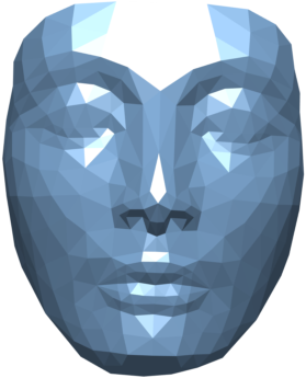
function P = PlotMesh(F,V)
e = ones(size(V,1),1);
Vrgb = [0.6*e, 0.8*e, e];
P = patch('Faces', F, 'Vertices', V, 'FaceVertexCData', Vrgb, 'EdgeColor', 'interp', 'FaceColor', 'interp');
shading interp
light('Position',[0, 1, 1]);
set(gcf, 'color', [0, 0, 0]);
view([0, 0, 1]);
axis equal off
load('Nefertiti.mat');
PlotMesh(F,V);
Vertex-Vertex Adjacency Matrix
The vertex-vertex adjacency matrix $A$ is defined by \begin{equation} A_{i,j} = \begin{cases} 1 &\mbox{if $[{v}_i,{v}_j]\in\mathcal{E}(\mathcal{M})$,}\\ 0 &\mbox{otherwise.} \end{cases} \end{equation}Construct the Vertex-Vertex Adjacency Matrix
VertexVertexAdjacency.m
function A = VertexVertexAdjacency(F)
Vno = max(F(:));
A = sparse(F, F(:,[2, 3, 1]), 1, Vno, Vno);
A = spones(A + A.');
load('Nefertiti.mat');
A = VertexVertexAdjacency(F);

% Plot the sparsity of the matrix A.
spy(A);
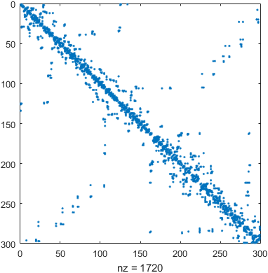
Exercise Find the set of neighboring vertices of the $53$th and $88$th vertices of the Nefertiti mesh model.
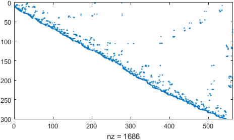
Vertex-Face Adjacency Matrix
The vertex-face adjacency matrix $G$ is defined by \begin{equation} G_{i,j} = \begin{cases} 1 &\mbox{if ${v}_i$ is a vertex of $j$-th face,}\\ 0 &\mbox{otherwise.} \end{cases} \end{equation}Construct the Vertex-Face Adjacency Matrix
VertexFaceAdjacency.m
function G = VertexFaceAdjacency(F)
Fno = size(F, 1);
Vno = max(F(:));
Fid = 1:Fno;
Fid = repmat(Fid, 1, 3);
G = sparse(F, Fid, 1, Vno, Fno);
load('Nefertiti.mat');

G = VertexFaceAdjacency(F);

spy(G);
The Edge Array
EdgeArray.m
function E = EdgeArray(F)
A = VertexVertexAdjacency(F);
[I, J] = find(triu(A));
E = [I, J];
Exercise Check the Euler characteristic $\chi=|V|-|E|+|F|$ of the Nefertiti mesh model.
Exercise Write a MATLAB function
VertexEdgeAdjacency.m for the construction of the vertex-edge adjacency matrix.
Exercise Write a MATLAB function
EdgeFaceAdjacency.m for the construction of the edge-face adjacency matrix.
Boundary Vertices
A vertex $v\in\mathcal{V}(\mathcal{M})$ is said to be a boundary vertex if $v\in\partial\mathcal{M}$.
load('Nefertiti.mat');

Vno = size(V, 1);
A = sparse(F, F(:,[2, 3, 1]), 1, Vno, Vno);
Gb = A - A.';
[Bi, Bj] = find( Gb == 1 );

PlotMesh(F, V);
hold on
plot3(V(Bi,1), V(Bi,2), V(Bi,3), 'g*');
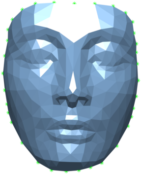
Check the order of the boundary vertices.
VBno = size(Bi,1);

PlotMesh(F, V);
set(gcf, 'color', [1, 1, 1]);
hold on
plot3(V(Bi,1), V(Bi,2), V(Bi,3), 'g*');
Vid = cellstr( num2str((1:VBno).') );
text(V(Bi,1), V(Bi,2), V(Bi,3)+1, Vid, 'VerticalAlignment', 'middle', 'HorizontalAlignment', 'center');
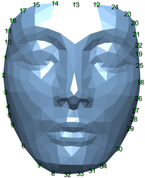
Exercise Reorder the indices of the boundary vertices in a counterclockwise order.
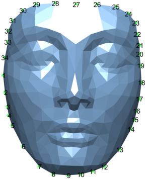
Check the order of the boundary vertices.
PlotMesh(F, V);
set(gcf, 'color', [1, 1, 1]);
hold on
plot3(V(VB,1), V(VB,2), V(VB,3), 'g*');
Vid = cellstr( num2str((1:VBno).') );
text(V(VB,1), V(VB,2), V(VB,3)+1, Vid, 'VerticalAlignment', 'middle', 'HorizontalAlignment', 'center');
The index set of the interior vertices can be obtained by a set operation.
Vno = size(V,1);
VI = setdiff((1:Vno).', VB);
Finally, we may write a MATLAB function for the ordered boundary indices of the triangular mesh as following.
BoundaryIndex.m
function [VB, VI] = BoundaryIndex(F)
Vno = max(max(F));
Gvv = sparse(F, F(:,[2 3 1]), 1, Vno, Vno);
Gb  = Gvv - Gvv.';
[Bi, Bj] = find( Gb == 1 );
VBno = size(Bi,1);
VB   = zeros(VBno, 1);
[bd_vertex, bd_ind] = min(Bi);
for jj = 1:VBno
    VB(jj) = bd_vertex;
    bd_ind = find( Bi == Bj(bd_ind) );
    bd_vertex = Bi(bd_ind);
    if ( bd_vertex == VB(1) ) && ( jj ~= VBno )
        VBno = jj;
        VB(jj+1:end) = [];
        break
    end
end
if nargout > 1
    VI = setdiff((1:Vno).', VB);
end
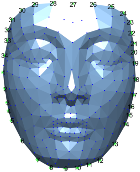
load('Nefertiti.mat');
[VB, VI] = BoundaryIndex(F);

PlotMesh(F, V);
set(gcf, 'color', [1,1,1]);
hold on
plot3(V(VB,1), V(VB,2), V(VB,3), 'g*');
plot3(V(VI,1), V(VI,2), V(VI,3), 'b.');
VBno = size(VB,1);
Vid = cellstr( num2str((1:VBno).') );
text(V(VB,1), V(VB,2), V(VB,3)+1, Vid, 'VerticalAlignment', 'middle', 'HorizontalAlignment', 'center');
OBJ Mesh File Format
The OBJ (.obj) format is a commonly used mesh file format which is supported by most of geometric processing softwares, e.g., MeshLab.Write OBJ Files
Output the mesh as an OBJ file.
function WriteOBJ(FileName, V, F)
if ~strcmpi(FileName(end-3:end), '.obj')
    FileName = [FileName '.obj'];
end
if size(V,2)==2
    V = [V, 0*V(:,1)];
end
fid = fopen(FileName,'wt');
fprintf(fid, 'v %f %f %f\n', V.');
fprintf(fid, 'f %d %d %d\n', F.');
fclose(fid);
load('Nefertiti.mat');

FileName = 'Nefertiti.obj';
WriteOBJ(FileName, V, F);